Model Checking Reward Markov Models with Uncertainties

Authors: Giovanni Bacci, Mikkel Hansen and, Kim G. Larsen

Affiliation: Department of Computer Science, Aalborg University, Denmark
e-mail: {giovbacci,mhan,kgl}@cs.aau.dk

We consider the problem of analysing Markov reward models (MRMs) in the presence of imprecise or uncertain rewards.
Properties of interests for their analysis are (i) probabilistic bisimilarity, and (ii) specifications expressed as probabilistic reward CTL formulae (PRCTL).
We consider two extensions of the notion of MRM, namely (a) constrained Markov reward models, i.e., MRMs with rewards parametric on a set variables subject to some constraints, and (b) stochastic Markov reward models, i.e., MRMs with rewards modelled as real-valued random variables as opposed to precise rewards.
Our approach is based on quantifier elimination for linear real arithmetic which is used for computing a symbolic representation of the set or parameter valuations satisfying a given property in the form of a quantifier-free first-order formula in the linear theory of the reals. Our work finds applications in model repair, where parameters need to be tuned so as to satisfy the desired specification, as well as in robustness analysis in the presence of stochastic perturbations.

Preliminaries

Markov Reward Models

In what follows we fix a finite set of atomic propositions AP

Definition (Markov chain) A Markov chain is a tuple M = (S, τ, l) consisting of a finite nonempty set of states S, a transition probability function τ : S → D(S), and a labeling function l : S → $2^{\mathrm{AP}}$ mapping states to atomic propositions.

The transition probability function can be equivalently represented as a state-indexed matrix ${\left(\tau \left(s\right)\left(t\right)\right)}_{s,t\in S}$. Analogously, the labeling function can be alternatively represented as a state-indexed vector. Later, we will use this alternative representation to express our models.

Definition (Markov reward model) A Markov reward model is a tuple R = (S, τ, l, ρ) where (S,τ,l) is a Markov chain, and ρ : S → R is the reward function assigning a reward to each state.

A Markov reward model probabilistically generates infinite paths in $S^{\omega }$ according to its underlying Markov chain; in addition, whenever a transition is performed, say from s to t, the system is rewarded by ρ(s). It is worth noting that the reward is given after leaving the current state.

Constrained Markov Reward Models

Constrained Markov reward models (CMRMs) model families of MRMs where both transition probabilities and state rewards are parametric on a set of real - valued variables subject to constraints expressed as a first-order formula in the linear theory of the reals.
Let x = ($x_1$,...,$x_k$) be a vector of real-valued parameters. We denote by E the set of affine maps f : ${\mathbb{R}}^k$ → R of the form f(x) = a . x + b where a ∈ ${\mathbb{Q}}^k$ and b ∈ Q.

Definition (constrained Markov reward model) A constrained Markov reward model is a tuple F = (S, τ, l, ρ, F) where S and l are defined as for Markov chains, τ : S → (S → E) is a parametric transition function, ρ : S → E is a parametric reward function, and F(x) is a linear first-order formula such that, for all s,t ∈ S, F(x) implies τ(s)(t) > 0 and  $\sum _{t\in S}\tau \left(s\right)\left(t\right)=1$.

Intuitively, a CMRM F = (S, τ, l, ρ, F) defines a family of MRMs arising by plugging in concrete values for the parameters. A parameter valuation v ∈ ${\mathbb{R}}^k$ is admissible (or feasible) if F(v) holds true.

Stochastic Markov Reward Models

It’s common practice to model experimental measurements by means of real-valued random variables distributed according to well studied families of distributions (e.g., normal or student’s T). Following this philosophy, we introduce the notion of stochastic Markov reward models (SMRMs) where state rewards are real-valued random variables.
Consider the probability space (Ω,Σ,P) representing the environment where the experiments are performed.  We will denote by Y the set of real-valued random variables of the form Y : Ω → R.

Definition (stochastic Markov reward model) A stochastic Markov reward model is a tuple J = (S, τ, l, ρ) where (S,τ,l) is a Markov chain and ρ : S → Y is a reward function assigning a real-valued random variables to each state.

An SMRM can be intuitively interpreted as a measurable function J : Ω → MRM where for a given event ω ∈ Ω, J(ω) is the MRM (S,τ, l, ${\rho }_{\omega }$) where ${\rho }_{\omega }$(s) = ρ(s)(ω) for all s ∈ S.

Quantifier Elimination for the linear theory real arithmetic

Mathematica implements a built-in quantifier elimination algorithm, called Resolve. However if the formula involves only  polynomials of degree one, we suggest the user to employ Mjollnir which implements more efficient methods.

Mjollnir is a tool developed by David Monniaux that implements quantifier elimination algorithm for the theory of linear real arithmetic. The tool is freely available at http://www-verimag.imag.fr/~monniaux/download/Mjollnir_2012-02-24.zip

Once installed you shall set the installation directory as done below.

$\mathrm{Options}\left[\mathrm{QE}\right]=\left\{\mathrm{Path}\to ''/Users/giovbacci/AAU/QuantifierElimination/Mjollnir/trunk/'',\mathrm{Method}\to ''Mjollnir''\right\};$

$\mathrm{QE}\left[\mathrm{expr\_},\mathrm{OptionsPattern}\left[\right]\right]:=\text{}\mathrm{If}[\mathrm{MatchQ}\left[\mathrm{OptionValue}\left[\mathrm{Method}\right],''Mjollnir''\right],\text{}\mathrm{Put}\left[\mathrm{expr},''temp.m''\right];\text{(*}\mathrm{export}\mathrm{the}\mathrm{expression}\mathrm{in}a\mathrm{temporary}\mathrm{file}\text{*)}\text{}\mathrm{Get}\left[''!''<>\mathrm{OptionValue}\left[\mathrm{Path}\right]<>''mjollnir\; --full-simplify\; temp.m''\right]\text{(*}\mathrm{execute}\mathrm{Mjollnir}\text{*)},\text{}\mathrm{Resolve}\left[\mathrm{expr},\mathrm{Reals}\right]\text{(*}\mathrm{execute}\mathrm{resolve}\text{*)}\text{}];$

Test

By default, quantifier elimination is performed using Mjollnir. Run the following test to check if Mjollnir works correctly.

${\forall }_z\left(\left(x\ge 0\left(x\ge 14\le x\&\&x\le 9\right)\&\&\left(x\le 05\le z\&\&z\le 10\right)\right)\&\&\left(x\le -1\left(x\ge 15\le z\&\&z\le 10\right)\&\&\left(x\le 03\le x\&\&x\le 5\right)\right)\right)$

$\left(x<0\&\&-1-x<0\right)||\left(-x<0\&\&-1+x<0\right)||\left(9-x\ge 0\&\&-4+x\ge 0\right)$

In case the test does not work you can set the Method as Automatic and use Resolve

$\mathrm{QE}\left[\mathrm{expr},\mathrm{Method}\to \mathrm{Automatic}\right]$

$\left(x<0\&\&-1-x<0\right)||\left(-1+x<0\&\&-x<0\right)||\left(-9+x\le 0\&\&4-x\le 0\right)$

Getting Started

Data Structures for CMRMs

A CMRMs are represented by means of (symbolic) terms of the form CMRM[S,tau,ell,rho,F]
The following definitions allow one to access each component of a given CMRM

The following definitions allow one to construct the underlying graph of a given CMRM.
The graph can be manipulated and visualized by using standard Mathematica functions for graphs.

$\text{(*}\mathrm{toGraph}\left[M:\mathrm{CMRM}\left[\mathrm{S\_},\mathrm{tau\_},\_,\_,\_\right]\right]:=\text{}\mathrm{Graph}\left[\left(\mathrm{DirectedEdge}@@\#\&\right)/@\left(\mathrm{Most}@\mathrm{ArrayRules}\left[\mathrm{tau}\right]⟦\mathrm{All},1⟧\right)\right];\text{*)}\text{}\mathrm{toGraph}\left[M:\mathrm{CMRM}\left[\mathrm{S\_},\mathrm{tau\_},\mathrm{ell\_},\mathrm{rho\_},\_\right]\right]:=\text{}\mathrm{Graph}\left[\mathrm{Labeled}\left[\mathrm{DirectedEdge}@@\#⟦1⟧,\#⟦2⟧\right]\&/@\left(\mathrm{Most}@\mathrm{ArrayRules}\left[\mathrm{tau}\right]\right),\text{}\mathrm{VertexSize}\to 0.3,\mathrm{VertexShapeFunction}\to ''Square'',\mathrm{VertexLabels}\to \mathrm{Table}\left[i\to \mathrm{Placed}\left[\left\{\mathrm{ell}⟦i⟧,\mathrm{rho}⟦i⟧,i\right\},\left\{\mathrm{Top},\mathrm{Bottom},\mathrm{Before}\right\}\right],\left\{i,\mathrm{Length}\left[S\right]\right\}\right]\right];\text{}\mathrm{Reachability}\left[M:\mathrm{CMRM}\left[\mathrm{S\_},\mathrm{tau\_},\_,\_,\_\right],\mathrm{u\_}\right]:=\text{}\mathrm{Append}\left[\mathrm{Select}\left[\mathrm{IncidenceList}\left[\mathrm{TransitiveClosureGraph}\left[\mathrm{toGraph}\left[M\right]\right],u\right],\#⟦1⟧⩵u\&\right]⟦\mathrm{All},2⟧,u\right];$

Declaration of CMRMs and SMRMs

A CMRM F = (S, τ, l, ρ, F) with S = {1,..,n} is represented by a term of the form CMRM[S,tau,ell,rho,F] where
- tau is an n × n probability matrix such that tau[[i,j]] = τ(i)(j), for all 1 ≤ i,j ≤ n,
- ell is a vector of length n such that ell[[i]] = l(i), for all 1 ≤ i ≤ n,
- rho is a vector of length n such that rho[[i]] = ρ(i), for all 1 ≤ i ≤ n.
- F is a first order formula in the linear theory of the reals.
Notably, parameters are implicitly represented by undeclared symbols.

Example: We are now ready to construct our first CMRM. We will model a gambler that tosses a coin according to the following rules.
Whenever the coin faces head, the following coin toss will give head again with probability q and tail with probability 1-q.
Whenever the coin faces tail, the following coin toss will fairly give head or tail with equal probability.
The reward gained after tossing is parametric on r . If the toss is done from head, then the reward is r-2, otherwise r+2.

We can visualize the above CMRM by plotting its underlying labeled graph.

$\mathrm{toGraph}\left[\mathrm{Coin}\right]$

An SMRM J = (S, τ, l, ρ) is represented by a term of the form SMRM[S,tau,ell,rho,decl] where S,tau, and ell are represented as for CMRMs and decl is a list of declarations of the form {x, distr} assigning each random variable x to its distribution. One can use any distribution provided in the Wolfram Language.

Example: Let us fix q = 1/2 and assume r to be a random variable distributed according to a Normal distribution with mean μ = 1 and standard deviation σ = 0.5. Accordingly, the gambler model described above can be rephrased as a SMRM as follows

Remark: we allow also to add constraints to the set of random rewards. These shall not be interpreted as feasibility constraints that restrict the set of possible outcomes. Rather, they should be interpreted as conditional constraints affecting the probability of our observations which will be conditioned under such constraints.
For instance, the above example can be extended by adding the constraint 0 ≤ r ≤ 2 indicating that we are interesting in observing the outcomes conditioned on the fact that the outcome for the random variable r lays in the closed interval [0,2].

Syntax for Probabilistic Reward CTL

PRCTL allows for state formulae describing properties about states in a MRM, and path formulae describing properties about paths in a MRM. State formulae Φ,Ψ and path formulae φ are constructed over the following abstract syntax:

Φ, Ψ  ::= True | False | AP[a] | Rew[rel, r] | Not[Φ] | Φ && Ψ | Φ || Ψ | Pr[J, X[Φ]] | Pr[J, U[Φ, Ψ] ] | Ex[R, Φ]

where a ∈ AP, r ∈ Q, rel ∈ {Equal, Less, LessEqual, Greater, GreaterEqual}, and J and R are intervals of the form Interval[{min,max}].

Model checking Constrained Markov Reward Models

Encoding PRCTL satisfiability

The following function implements the encoding of the PRCTL model checking problem for CMRMs.

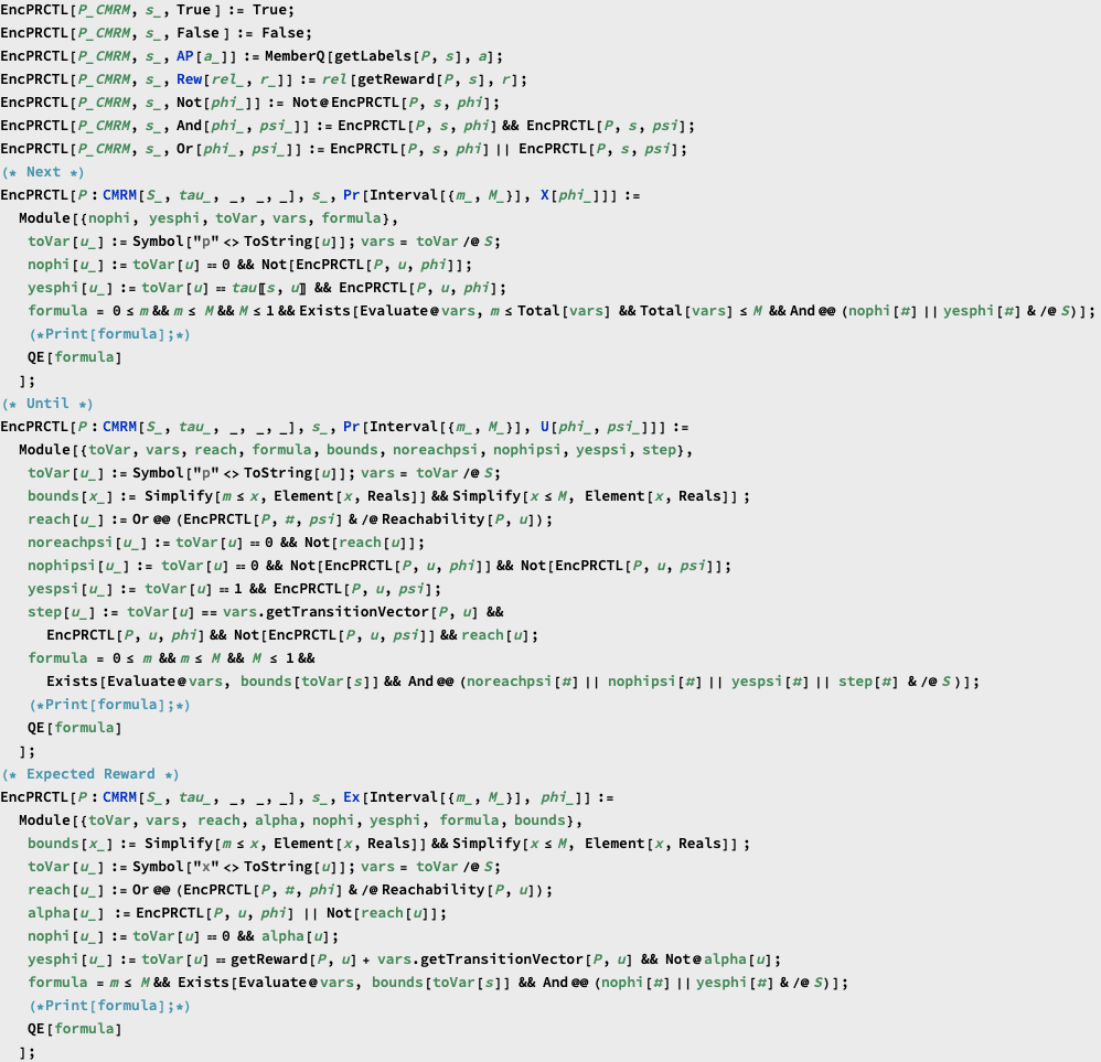
Model checking CMRMs against PRCTL

$\mathrm{Models}\left[\mathrm{P\_CMRM},\mathrm{s\_},\mathrm{Phi\_},\mathrm{opt}:\mathrm{OptionsPattern}\left[\right]\right]:=\text{}\mathrm{Module}\left[\left\{\mathrm{tp},\mathrm{satformula}\right\},\text{}\left\{\mathrm{tp},\mathrm{satformula}\right\}=\mathrm{Timing}\left[\mathrm{QE}\left[\mathrm{EncPRCTL}\left[P,s,\mathrm{Phi}\right]\&\&\mathrm{getConstraints}\left[P\right]\right]\right];\text{}\mathrm{If}\left[\mathrm{OptionValue}\left[\mathrm{Verbose}\right],\text{}\mathrm{Print}\left[''Computation\; time:'',\mathrm{tp},''sec''\right];\text{}\right];\text{}\mathrm{satformula}\text{}\right];$

Model checking Stochastic Markov Reward Models

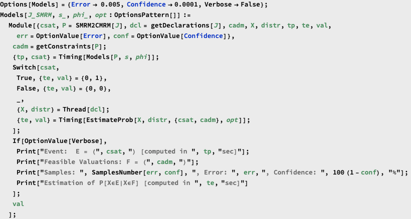
Model Checking of Stochastic Markov Reward Models

Monte Carlo Estimation

Number of samples based on the Chernoff bound

$\mathrm{SamplesNumber}\left[\mathrm{err\_},\mathrm{conf\_}\right]:=\mathrm{Ceiling}\left[-\mathrm{Log}\left[\mathrm{conf}/2\right]/\left(2\mathrm{err}^2\right)\right];$

Estimate the event by sampling the random variables

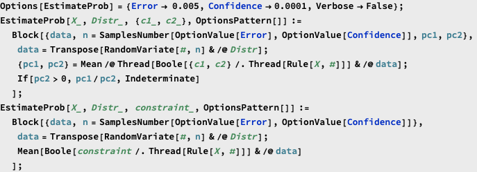
Model Checking SMRMs against PRCTL

$\mathrm{getDeclarations}\left[\mathrm{J\_SMRM}\right]:=\mathrm{Last}\left[J\right];$

Examples

Modelling the stress level of a PhD student

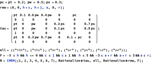
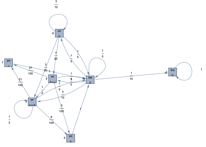
Consider the following CMRM modelling the stress level of a Ph.D. student in computer science. It has seven states, namely $s_1$, . . . , $s_7$, annotated with the propositions “thk” (thinking), “ths” (thesis), “wr” (writing paper), “tc” (tool coding), and “pe” (paper evaluation). The level of stress of the student is modelled by associating with each state a reward that represents the stress that the student accumulates in the state at each time unit. After spending some time thinking, the student starts developing a tool with probability pc = 0.2, or writing a paper with probability pw = 0.5 (40% of the times for a journal and 60% for a conference), otherwise the student submits the thesis with probability 0.1. Once the tool is mature enough, the student starts writing a paper about it with probability pw (70% of which for a journal, otherwise for a conference). When a paper has been completed it is submitted for evaluation with probability ps = 0.3. The paper may be rejected or accepted (moving resp. to s7 or s5) according to some acceptance rate. At any moment before the thesis is completed, the student may move back to s1 with probability pt = 0.2 to think on how to proceed with his/her Ph.D.
State rewards are parametric on h, c, j, a, and r. Here, the parameter h models the help of the supervisor, whereas c and j represent the stress that accumulates while writing a conference paper c, or a journal paper j. The stress caused by having a paper accepted or rejected in modelled by the parameters a and r respectively. These parameters are subject to the constraints F defined below.  

$\mathrm{toGraph}\left[R\right]$

We can express the property “the average level of stress accumulated by the student until the thesis is submitted doesn’t exceed 10” as the following PRCTL formula

$\mathrm{phi1}=\mathrm{Ex}\left[\mathrm{Interval}\left[\left\{0,10\right\}\right],\mathrm{AP}\left[''ths''\right]\right];$

Analogously, we can express the property “the student completes the thesis without passing through a state with stress level higher than 2 with probability greater than or equal to 0.5” by means of the following formula

$\mathrm{phi2}=\mathrm{Pr}\left[\mathrm{Interval}\left[\left\{0.5,1\right\}\right],U\left[\mathrm{Rew}\left[\mathrm{LessEqual},2\right],\mathrm{AP}\left[''ths''\right]\right]\right];$

The set of feasible valuations satisfying the first formula can be modeled as the following expression.

$\mathrm{FullSimplify}@\mathrm{Models}\left[R,1,\mathrm{phi1},\mathrm{Verbose}\to \mathrm{True}\right]$

$\text{Computation time:}\text{}0.016616\text{}\sec$

$-5\le h\le 0\&\&c\le j\&\&0\le 57a+575c+750h+175j+168r\le \frac{1750}{3}\&\&a\le r\&\&-3\le a+r\le 3\&\&c\ge 1$

Analogously, the set of feasible valuations satisfying the second formula are

$\mathrm{FullSimplify}@\mathrm{Models}\left[R,1,\mathrm{phi2},\mathrm{Verbose}\to \mathrm{True}\right]$

$\text{Computation time:}\text{}0.01222\text{}\sec$

$-5\le h\le 0\&\&c\le j\&\&a\le r\&\&-3\le a+r\le 3\&\&c\ge 1$

Remark: our encoding allows one to have parameters in the formula. This feature can be used to express families of properties, but also to relate the probability of satisfying one formula with that of satisfying another one.
For instance, one can express complex properties such as “the student completes the thesis without passing through a state with stress level higher than x+2 with probability greater than or equal to x and can also complete the thesis without passing through a state with stress level higher than x+1 with probability smaller than or equal to x”.

$\mathrm{FullSimplify}@\mathrm{Models}\left[R,1,\mathrm{phi3}\&\&\mathrm{phi4},\mathrm{Verbose}\to \mathrm{True}\right]$

$\text{Computation time:}\text{}0.020978\text{}\sec$

$5+h\ge 0\&\&h\le 0\&\&a+r\le 3\&\&\left(\left(c\le j\&\&\left(\left(3+a+r\ge 0\&\&\left(\left(a\le r\&\&\left(\left(c+h>\frac{59}{52}\&\&52x⩵7\right)||\left(c\ge 1\&\&\left(\left(h+j\le \frac{219}{97}\&\&97r>122\&\&97x⩵25\right)||\left(h+j\le 3\&\&r\le 3\&\&x⩵1\right)||\left(h+j\le 2+x\&\&\left(\left(h+j>1+x\&\&\left(\left(97x\le 25\&\&\left(4x\ge 1||\left(r>1+x\&\&136x\ge 25\right)\right)\right)||\left(4x\ge 1\&\&r\le 2+x\&\&x\le 1\right)\right)\right)||\left(r\le 2+x\&\&r>1+x\&\&x\le 1\&\&97x>25\right)\right)\right)\right)\right)||\left(c+h>1+x\&\&52x>7\&\&\left(\left(h+j\le 2+x\&\&\left(97x\le 25||\left(r\le 2+x\&\&x\le 1\right)\right)\right)||\left(c+h\le 2+x\&\&\left(136x\le 25||\left(r\le 2+x\&\&4x\le 1\right)\right)\right)\right)\right)\right)\right)||\left(c\ge 1\&\&\left(\left(h+j\le \frac{219}{97}\&\&97r>219\&\&97x⩵25\right)||\left(h+j\le 2+x\&\&r\le 2+x\&\&r>1+x\&\&x\le 1\&\&346x>175\right)\right)\right)\right)\right)||\left(c\ge 1\&\&a\le r\&\&a>1+x\&\&h+j\le 2+x\&\&\left(34x\ge 7||\left(h+j>1+x\&\&212x\ge 35\right)\right)\right)\right)\right)||\left(c\ge 1\&\&a\le r\&\&\left(\left(3+a+r\ge 0\&\&\left(\left(c+h\le \frac{9}{4}\&\&h+j>\frac{9}{4}\&\&4r\le 9\&\&4x⩵1\right)||\left(c+h\le \frac{297}{136}\&\&h+j>\frac{297}{136}\&\&136r>161\&\&136x⩵25\right)||\left(c+h\le 2+x\&\&h+j>2+x\&\&r\le 2+x\&\&r>1+x\&\&4x\le 1\&\&136x>25\right)\right)\right)||\left(a>1+x\&\&c+h\le 2+x\&\&h+j>2+x\&\&808x\le 175\&\&212x\ge 35\right)\right)\right)\right)$

Assume now that in the model described above, we interpret the parameters h, c, j, a, and r as pairwise independent random variables distributed according to the following declaration

We can now estimate the probability of satisfying the formula phi1

$N@\mathrm{Models}\left[J,1,\mathrm{phi1},\mathrm{Verbose}\to \mathrm{True}\right]$

$\text{Event: E = (}\text{}57a+575c+750h+175j+168r\ge 0\&\&1750-171a-1725c-2250h-525j-504r\ge 0\text{}\text{) [computed in}\text{}0.009605\text{}\text{sec]}$

$\text{Feasible Valuations: F = (}\text{}\mathrm{True}\text{})$

$\text{Samples:}\text{}198070\text{}\text{, Error:}\text{}0.005\text{}\text{, Confidence:}\text{}99.99\text{}\%$

$\text{Estimation of P[X∈E|X∈F] [computed in}\text{}4.035516\text{}\text{sec]}$

$0.15636896046852122$

The SMRM above does not consider the feasibility constraints F used above. We add such constraints as follows.

$\text{Event: E = (}\text{}-h\ge 0\&\&-c+j\ge 0\&\&57a+575c+750h+175j+168r\ge 0\&\&-a+r\ge 0\&\&1750-171a-1725c-2250h-525j-504r\ge 0\&\&5+h\ge 0\&\&3+a+r\ge 0\&\&3-a-r\ge 0\&\&-1+c\ge 0\text{}\text{) [computed in}\text{}0.007937\text{}\text{sec]}$

$\text{Feasible Valuations: F = (}\text{}-5\le h\&\&h\le 0\&\&c\le j\&\&c\ge 1\&\&h\le 5\&\&-3\le a+r\&\&a+r\le 3\&\&a\le r\text{})$

$\text{Samples:}\text{}198070\text{}\text{, Error:}\text{}0.005\text{}\text{, Confidence:}\text{}99.99\text{}\%$

$\text{Estimation of P[X∈E|X∈F] [computed in}\text{}8.958402\text{}\text{sec]}$

$0.15567282321899736$

Queueing Model

$\text{Computation time:}\text{}0.00867\text{}\sec$

$\frac{10205}{43}\le 71l+580r\le \frac{20410}{43}$