The MDPDist Mathematica package
On-the-fly exact computation of bisimilarity distances for Markov Decision Process with rewards
Authors: Giorgio Bacci, Giovanni Bacci, Kim G. Larsen, and Radu Mardare
In this tutorial we present the main features of the MDPDist package. This Mathematica package implements an on-the-fly method for computing the bisimilarity pseudometric of Ferns et al. [1] for Markov Decision Process with rewards. The algorithm implemented in this package is an exension of the on-the-fly method recently proposed in [2] for Markov Chains.
Preliminaries
Markov Decision Processes and Bisimulation
A probability distribution over a nonempty enumerable set S is a function μ : S → [0,1] such that ![]() . We denote by Δ(S) the set of probability distributions over S.
. We denote by Δ(S) the set of probability distributions over S.
Definition (Markov Decision Process). A Markov Decision Process with rewads (MDP) is a tuple M =(S,A,τ,ρ) consisting of a finite nonempty set S of states, a finite nonempty set A of actions, a transition function τ : S × S → Δ(S), and a reward function τ ∶ S × A → R.
The operational behavior of an MDP M =(S,A,τ,ρ) is as follows: the process in the state ![]() chooses nondeterministically an action a ∈ A and it changes the state to
chooses nondeterministically an action a ∈ A and it changes the state to ![]() , with the probabilty τ(
, with the probabilty τ(![]() ,a)(
,a)(![]() ). The choice of the action a made in
). The choice of the action a made in ![]() is rewarded by ρ(
is rewarded by ρ(![]() ,a). The exectutions are transition sequences w = (
,a). The exectutions are transition sequences w = (![]() ,
,![]() ),(
),(![]() ,
,![]() ),....; the challenge is to find strategies for choosing the actions in order to maximize the accumulated reward
),....; the challenge is to find strategies for choosing the actions in order to maximize the accumulated reward ![]() , where λ ∈ (0,1) is the discount factor. A strategy is given by a function π : S → Δ(A), called policy, where π(
, where λ ∈ (0,1) is the discount factor. A strategy is given by a function π : S → Δ(A), called policy, where π(![]() )(a) is the probabilty distribution over executions defined, for arbitrary w = (
)(a) is the probabilty distribution over executions defined, for arbitrary w = (![]() ,
,![]() ),(
),(![]() ,
,![]() )...., by
)...., by ![]() . The value of s according to π is characterized by
. The value of s according to π is characterized by ![]() , where Ω(w) is the set of executions from s.
, where Ω(w) is the set of executions from s.
Definition (Stocastic Bisimulation). Let M =(S,A,τ,ρ) be an MDP. An equivalence relation R ⊆ S × S is a stocatic bisimulation if whenever (s,t) ∈ R then, for all a ∈ A, ρ(s,a) = ρ(t,a) and, for all R-equivalence classes C, ![]() . Two states s,t ∈ S are stocatic bisimilar, written s ∼ t, if they are related by some stochastic bisimulation on M.
. Two states s,t ∈ S are stocatic bisimilar, written s ∼ t, if they are related by some stochastic bisimulation on M.
Bisimilarity Pseudometric
To cope with the problem of measuring how similar two MDPs are, Ferns et al. [1] defined a bisimilarity pseudometric that measures the behavioral similarity of two non-bisimilar MDPs. This is defined as the least fixed point of a transformation operator on functions in S × S → [0,∞).
Consider an arbitrary MDP M =(S,A,τ,ρ) and a discount factor λ ∈ (0,1). The set S × S → [0,∞) of [0,∞)-valued maps on S × S equipped with the point-wise partial order defined by d ⊆ d’ ⇔ d(s,t) ≤ d’(s,t), for all s,t ∈ S.
We define a fixed point operator ![]() , for d : S × S → [0,∞) and s,t ∈ S as
, for d : S × S → [0,∞) and s,t ∈ S as
![]()
Where ![]() denotes the optimal value of a Transportation Problem with marginals τ(s,a) and τ(t,a) and costs given by d
denotes the optimal value of a Transportation Problem with marginals τ(s,a) and τ(t,a) and costs given by d
![]()
![]() is monotonic, thus, by Tarski’s fixed point theorem, its admits a least fixed point. This fixed point is the bisimilarity pseudometric.
is monotonic, thus, by Tarski’s fixed point theorem, its admits a least fixed point. This fixed point is the bisimilarity pseudometric.
Definition (Bisimilarity psudometric). Let M =(S,A,τ,ρ) be an MDP and λ ∈ (0,1) be a discount factor, then the λ-discounted bisimilarity pseudometric for M, written ![]() , is the lest fixed point of
, is the lest fixed point of ![]() .
.
The pseudometric ![]() enjoys the property that two states are at distance zero if and only if they are bisimilar.
enjoys the property that two states are at distance zero if and only if they are bisimilar.
Getting started
The package can be loaded by setting as current directory the directory of the MDPDist package, then using the commad << (Get) as follows
![]()
Encoding and manipulating Markov Decision Processes
Encoding an MDP
An MPD M =(S,A,τ,ρ) with ![]() and
and ![]() is represented as a term of the form MPD[tm,rw,act] where
is represented as a term of the form MPD[tm,rw,act] where
- tm is an n × m × n probability matrix such that tm[[i,k,j]] = ![]() for all 1 ≤ i,j ≤ n and all 1 ≤ k ≤ m,
for all 1 ≤ i,j ≤ n and all 1 ≤ k ≤ m,
- rw is an n × m real-valued matrix such that rw[[i,k]]= ![]() for all 1 ≤ i ≤ n and all 1 ≤ k ≤ m, and
for all 1 ≤ i ≤ n and all 1 ≤ k ≤ m, and
- act is a list of pairwise distinct strings such that act[[k]] represents the action ![]() for all 1 ≤ k ≤ m.
for all 1 ≤ k ≤ m.
A state ![]() is implicitly represented by its index 1 ≤ i ≤ n.
is implicitly represented by its index 1 ≤ i ≤ n.
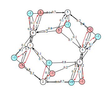
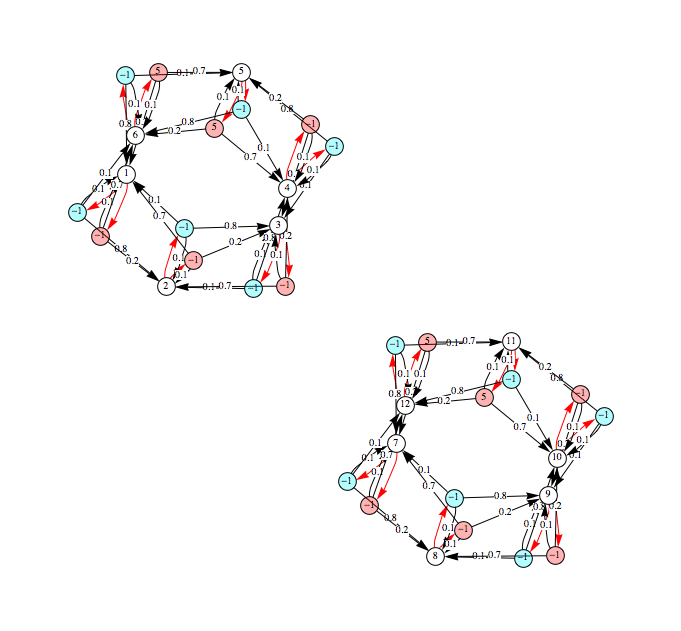
Assume we want to encode the following MDP M =(S,A,τ,ρ) with S = {1,2,3,4,5,6} and A = {inc, dec}, with the following intuitive operational behavior. Given M in state i, the choice of the action inc causes the MDP to move in state i+1 with probability 0.8, and to stay in state i or to move in state i-1 both with probability 0.1. The choice of the action dec causes the MDP to move in state i-1 with probability 0.7, to stay in state i with probability 0.1, and to move in state i+1 with probability 0.2. The reward of choising an inc action is always -1, whereas the reward for a dec action is 5 if it is made from state 5 or 6, 0 otherwise.
Mathematica allows to easily define functions and lists, so that we can exploit these features in order to define the data structures that are needed to encode M
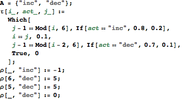
A represents the set of actions, τ is the transition function and ρ is the reward function.
One can obtain the respective transition and reward matrix using the built-in function Table as follows:
![]()
![]()
![]()
Then M is encoded by
![]()
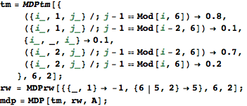
Alternatively, one may use the functions MDPtm and MDPrw to construct the transition and the reward matrices listing only the values different from zero. Given the list of rules tmRules = { ![]() , the probabilty transition matrix induced by the probability transition function τ may be constructed by calling MDPtm[tmRules, n, m].
, the probabilty transition matrix induced by the probability transition function τ may be constructed by calling MDPtm[tmRules, n, m].
Analogously, for rwRules = { ![]() , one can construct the reward matrix induced by the reward function ρ by calling MDPrw[rwRules, n, m].
, one can construct the reward matrix induced by the reward function ρ by calling MDPrw[rwRules, n, m].
The list of rules may be given explicitly or using patterns. For example, the matrices tm and rw defined above can be constructed as follows
Manipulating MDPs
An MDP is dispayed by the function PlotMDP. States are represented as white nodes labeled with their respective index. Red edges exiting from each node represent a nondeterministic choice of an action. The chosen action is displayed as a colored node labeled with its associated reward, called choice node. Edges exiting form a choice node represent the probability distribution obtained after a nondeterministic choice. For example, the MDP mdp defined above is dispayed as follows
![]()
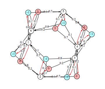
Given a sequence ![]() of MDPs, JoinMDP[
of MDPs, JoinMDP[![]() ] yields an MDP representing their disjoint union, where the indices representing the set of states are obtained shifting the indices of the states of its arguments according to their relative order in the sequence (e.g. if
] yields an MDP representing their disjoint union, where the indices representing the set of states are obtained shifting the indices of the states of its arguments according to their relative order in the sequence (e.g. if ![]() has n states, the index corresponding to the i-th state of
has n states, the index corresponding to the i-th state of ![]() in JoinMDP[
in JoinMDP[![]() ,
,![]() ] is n + i).
] is n + i).
![]()
Computing Bisimilarity Distances
Given an MDP M, a discount factor λ, and a list of state pairs Q, BDistMDP[M,λ,Q] computes the distance ![]() associated with each pair of states (s,t) in Q. For example, taking MDP mdp considered so far, a discount factor 0.5 and a single-pair query Q = {(1,2)} we have
associated with each pair of states (s,t) in Q. For example, taking MDP mdp considered so far, a discount factor 0.5 and a single-pair query Q = {(1,2)} we have
![]()
![]()
while for the query Q = {(1,2),(3,4),(6,5)} we have
![]()
![]()
If one is interested in computing the distance between all state pairs, it can use the alias All as follows
![]()

The computation can be traced setting the option Verbose to True. It will display the couplings encoutered during each iteration of the on-the-fly algorithm. This option can be also used to analyze how the algorithm explores the state space of the MDP.
![]()
![]()
![]()
![]()


![]()
![]()
![]()


![]()
![]()
![]()


![]()
![]()
![]()


![]()
![]()
![]()


![]()
![]()
![]()


![]()
![]()
![]()


![]()
![]()
![]()


![]()
![]()
![]()


![]()
![]()
![]()


![]()
![]()
![]()


![]()
![]()
![]()

One can provide some estimates in order to further reduce the exploration of the state space. This can be done using the option Estimates
![]()

Exact Computations
Mathematica allows one to perform exact computations over Rational numbers. Usually the Bellman-optimality equation system is computed approximately since it is in general a non-linear equation system. Despite this fact, our method is able to compute the exact result when the input MDP is rational-valued (i.e. both the transition fuction and the reward function are rational-valued)
For example, the MDP we considered so far can be rationalized as follows
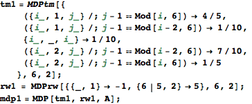
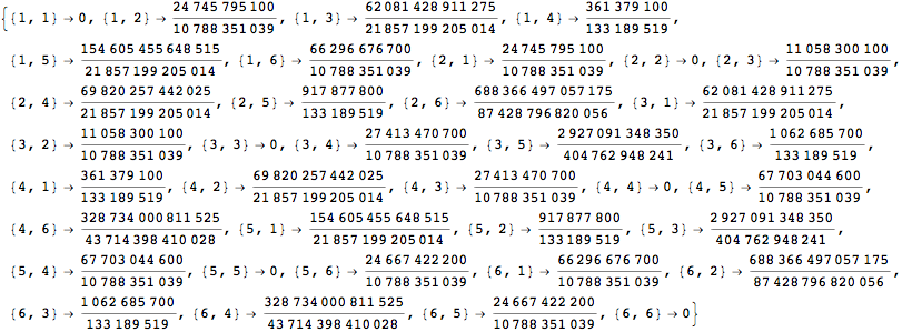
now, the exact value of the distance can be computed setting the option Exact to True
![]()
Bisimilarity Classes & Quotient
Due to the fact that ![]() (s,t) equals zero if and only if the states s and t are bisimilar, we can use the algorithm for computing
(s,t) equals zero if and only if the states s and t are bisimilar, we can use the algorithm for computing ![]() in order to compute the bisimilarity classes and the bisimilarity quotient for an MDP.
in order to compute the bisimilarity classes and the bisimilarity quotient for an MDP.
The function BisimClassesMDP[M] returns the set of bisimilarity classes of M, that is S/∼.
![]()
![]()
![]()
![]()
The function BisimQuotientMDP[M] yields an MDP representing the bisimilarity quotient of M.
![]()
