The MCDist Mathematica package
On-the-fly exact computation of bisimilarity distances for Markov Chains
Authors: Giorgio Bacci, Giovanni Bacci, Kim G. Larsen, and Radu Mardare
In this tutorial we present the main features of the MCDist package. This Mathematica package implements an on-the-fly method for computing the bisimilarity pseudometric of Desharnais et al. [1] for Markov Chains. The algorithm implemented in this package is based on the technique recently proposed in [2].
Preliminaries
Markov Chains and Probabilistic Bisimulations
Definition (Markov Chain). A (discrete-time) Markov chain (MC) is a tuple M = (S, Σ, π, ℓ) consisting of a finite nonempty set S of states, a nonempty set A of labels, a transition probability function π : S × S → [0,1] such that, for arbitrary s ∈ S, ![]() , and a labelling function ℓ : S → Σ.
, and a labelling function ℓ : S → Σ.
From a theoretical point of view, it is irrelevant whether the transition probability function of a given MC has rational values or not, However, for algorithmic purposes, here we assume that for arbitrary s,t ∈ S, π(s,t) ∈ Q ∩ [0,1].
Definition (Probabilistic Bisimulation). Let M = (S, Σ, π, ℓ) be an MC. An equivalence relation R ⊆ S × S is a probabilistic bisimulation if whenever (s,t) ∈ R, ℓ(s) = ℓ(t) and for each R-equivalence class C, ![]() .
.
Two states s,t ∈ S are bisimilar, written s ∼ t, if they are related by some probabilistic bisimulation.
Bisimilarity Pseudometric
The notion of equivalence can be relaxed by means of a pseudometric, which tells us how far apart from each other two elements are and whenever they are at zero distance they are equivalent. Desharnais et al. [1] defined a bisimilarity pseudometric that measures the behavioral similarity of two non-bisimilar MCs. In [3], van Breugel et al. characterized this pseudometric as the least fixed point of a operator on functions in S × S → [0,1].
Consider an MC M = (S, Σ, π, ℓ) and a discount factor λ ∈ (0,1]. The set S × S → [0,1] of [0,1]-valued maps on S × S equipped with the point-wise partial order defined by d ⊆ d’ ⇔ d(s,t) ≤ d’(s,t), for all s,t ∈ S.
We define a fixed point operator ![]() , for d : S × S → [0,1] and s,t ∈ S as
, for d : S × S → [0,1] and s,t ∈ S as
![]()
Where ![]() denotes the optimal value of a Transportation Problem with marginals π(s,·) and π(t,·) and costs given by d
denotes the optimal value of a Transportation Problem with marginals π(s,·) and π(t,·) and costs given by d
![]()
![]() is monotonic, thus, by Tarski’s fixed point theorem, its admits a least fixed point. This fixed point is the bisimilarity pseudometric.
is monotonic, thus, by Tarski’s fixed point theorem, its admits a least fixed point. This fixed point is the bisimilarity pseudometric.
Definition (Bisimilarity psudometric). Let M = (S, Σ, π, ℓ) be an MC and λ ∈ (0,1] be a discount factor, then the λ-discounted bisimilarity pseudometric for M, written ![]() , is the least fixed point of
, is the least fixed point of ![]() .
.
The pseudometric ![]() enjoys the property that two states are at distance zero if and only if they are bisimilar.
enjoys the property that two states are at distance zero if and only if they are bisimilar.
Getting started
The package can be loaded by setting as current directory that of the MCDist package, then using the commad << (Get) as follows
![]()
Encoding and manipulating Markov Chains
An MC M = (S, Σ, π, ℓ) with ![]() is represented by a term of the form MC[tm, lbl] where
is represented by a term of the form MC[tm, lbl] where
- tm is an n × n probability matrix such that tm[[i,j]] = ![]() , for all 1 ≤ i,j ≤ n,
, for all 1 ≤ i,j ≤ n,
- lbl is a list of strings (or integers) such that lbl[[i]] = ℓ(![]() ) for all 1 ≤ i ≤ n.
) for all 1 ≤ i ≤ n.
A state ![]() is implicitly represented by its index 1 ≤ i ≤ n.
is implicitly represented by its index 1 ≤ i ≤ n.
For example we can encode an MC by defining tm and lbl as follows:
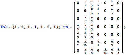
Then, the MC can be displayed by means of its undelying graph. Labels are displayed using different colors.
![]()
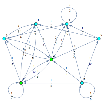
Alternatively, one may use the functions MCtm to construct the transition matrix, listing only the values different from zero. Given the list of rules tmRules = { ![]() , the probabilty transition matrix induced by the probability transition function π may be constructed by calling MCtm[tmRules, n].
, the probabilty transition matrix induced by the probability transition function π may be constructed by calling MCtm[tmRules, n].
The list of rules may be given explicitly or using patterns. For example, the matrix tm defined above can be constructed as follows

![]()
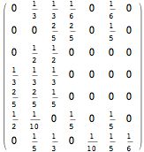
One can check that M is a well-formed MC by calling MCQ[M]
![]()
![]()
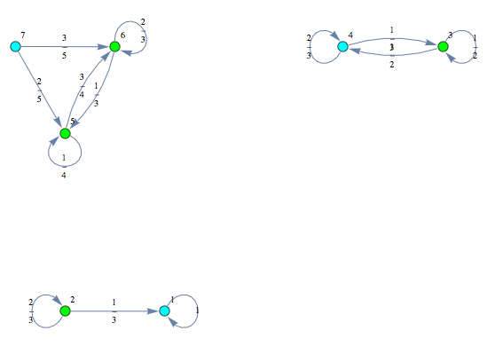
Given a sequence of Markov chains ![]() , one may construct their disjoint union using the function JoinMC
, one may construct their disjoint union using the function JoinMC

Run the on-the-fly algorithm
Given a MC M = MC[π,ℓ], a discount factor λ ∈ (0,1], and a list of pairs of states Q, the bisimilarity distance between the pairs in Q is computed by calling the function BDistMC as follows
![]()
![]()
The Verbose option may be used to trace the computation steps
![]()
![]()
![]()
![]()


![]()
![]()
![]()
![]()

![]()
![]()
![]()
![]()

![]()
![]()
![]()
![]()
![]()
For computing the distance between all pair of states one can use as query list the alias All
![]()

The output is returned as a set of ArrayRules, so that one can easily transform it into a matrix using the function SparseArray
![]()
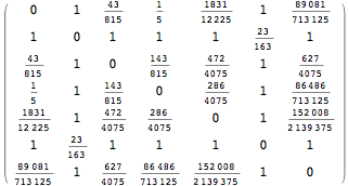
Bisimilarity Distance and Bisimilarity Quotient
Due to the fact that ![]() (s,t) equals zero if and only if the states s and t are bisimilar, the algorithm for computing
(s,t) equals zero if and only if the states s and t are bisimilar, the algorithm for computing ![]() can be used to compute the bisimilarity classes and the bisimilarity quotient for an MC.
can be used to compute the bisimilarity classes and the bisimilarity quotient for an MC.
Let M = (S, Σ, π, ℓ) be a (psedo-randomly generated) Markov chain with 50 states and outer-degree 2
![]()
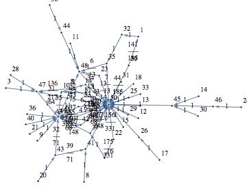
The function BisimClassesMC[M] returns the set of bisimilarity classes of M, that is S/∼.
![]()
![]()
so that this can be used to construct an MC M’ bisimilar to M with all the states that are bisimilar in M lumped together. M’ is also known as the bisimilar quotient of M.
![]()
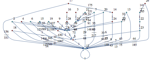
Examples
Example 1
Here we present an example taken from [2], which shows most of the features of the on-the-fly algorithm.
Consider the following MC:

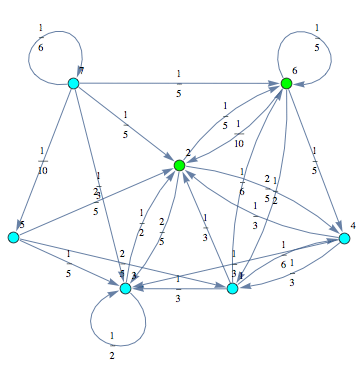
Let us compute the undiscouted distance between the state ![]() and
and ![]() , namely
, namely ![]()
![]()
![]()
![]()
![]()

![]()
![]()
![]()
![]()
![]()
![]()
![]()
![]()
![]()
![]()
![]()
![]()
![]()
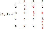
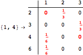
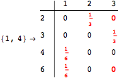
Looking at the execution trace we see that during the computation of d(1,4) an over-approximation for the distance d(3,4) is computed.
This happens because we encountered a coupling that demands d(3,4) for computing an over-approximation of d(1,4).
However, the first improvement of the current coupling makes the computation of d(3,4) no more demanded for d(1,4), so that no further improvement on (3,4) is made.
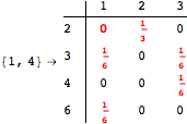
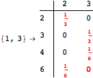
The following execution trace shows that the exact computation of ![]() demands an exact computation of
demands an exact computation of ![]() ,
, ![]() and
and ![]()
![]()
![]()
![]()
![]()

![]()
![]()
![]()
![]()


![]()
![]()
![]()
![]()


![]()

![]()
![]()



![]()

![]()
![]()


![]()

![]()
![]()
![]()
One would claim that if we ask for the exact computation of d(3,4), d(1,4) and d(2,6) the computation will do the same steps made for d(3,4). However, the exact computation of d(1,4) does not need an exact computation of the remaining pairs.
Thus, considering the pair (1,4) before (3,4) will allow us to reduce the size of the linear equation systems computed for d(3,4).
![]()
![]()
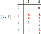
Another way to reduce the exploration of the MC is to give estimates for some distances. Assume we have an over-approximation of the exact value for d(2,6). By using this information, we can further reduce the state space explotation of the MC. This is done using the Estimates option as follows:
![]()
![]()
![]()
![]()

![]()
![]()
![]()
![]()

![]()
![]()
![]()
![]()


![]()
![]()
![]()
![]()
![]()
Using the estimate ![]() for the distance d(2,6) we had considerably reduced the number of steps for computing a good over-approximation for d(3,4).
for the distance d(2,6) we had considerably reduced the number of steps for computing a good over-approximation for d(3,4).
The Craps Game
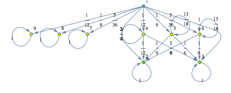
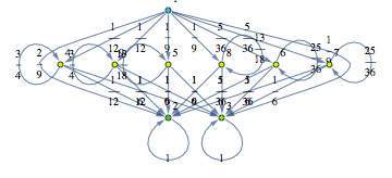
Here we present two different MCs modeling slightly different versions for the “craps game” (these are taken from the book Principles of Model Checking, Examples 10.4 and 10.23). We compare the two MCs by means of the distance beteween their initial states.

![]()

![]()
![]()
![]()