The MCApprox Mathematica package
Metric-based State Space Reduction for Markov Chains
Authors: Giovanni Bacci, Giorgio Bacci, Kim G. Larsen, and Radu Mardare
In this tutorial we present the main features of the MCApprox package. This Mathematica package implements an Expectation Maximization method for finding a “good” k-states approximation of any given Markov chain. Here bu “good” we mean that it behavior is certified to be close to the original Markov chain by measn of the bisimilarity pseudometric of Desharnais et al. [1].
Preliminaries
Markov Chains and Probabilistic Bisimulations
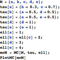
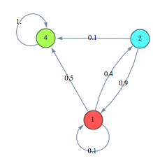
Definition (Markov Chain). A (discrete-time) Markov chain (MC) is a tuple M = (M,τ, ℓ) consisting of a finite nonempty set M of states, a transition probability function τ : M → Distr(M) (i.e., for arbitrary m ∈ M, ![]() ), and a labelling function ℓ : M → L. Where L is a coutable set of labels.
), and a labelling function ℓ : M → L. Where L is a coutable set of labels.
From a theoretical point of view, it is irrelevant whether the transition probability function of a given MC has rational values or not, However, for algorithmic purposes, here we assume that for arbitrary m,u ∈ M, τ(m,u) ∈ Q ∩ [0,1].
Definition (Probabilistic Bisimulation). Let M = (M,τ, ℓ) be an MC. An equivalence relation R ⊆ M × M is a probabilistic bisimulation if whenever (m,u) ∈ R, ℓ(m) = ℓ(u) and for each R-equivalence class C, ![]() .
.
Two states m,u ∈ M are bisimilar, written m ∼ u, if they are related by some probabilistic bisimulation.
Bisimilarity Pseudometric
The notion of equivalence can be relaxed by means of a pseudometric, which tells us how far apart from each other two elements are and whenever they are at zero distance they are equivalent. Desharnais et al. [1] defined a bisimilarity pseudometric that measures the behavioral similarity of two non-bisimilar MCs. In this tutorial we present this distance by means of its fixed point characterization given by van Breugel et al. [3].
Consider an MC M = (M,τ, ℓ) and a discount factor λ ∈ (0,1]. The set M × M → [0,1] of [0,1]-valued maps on M × M equipped with the point-wise partial order defined by d ⊆ d’ ⇔ d(m,u) ≤ d’(m,u), for all m,u ∈ S.
We define a fixed point operator ![]() , for d : M × M → [0,1] and m,u ∈ S as
, for d : M × M → [0,1] and m,u ∈ S as
![]()
Where ![]() deonted the Kantorivich pseudometric over probability distributions in M with underlying space distance d. One may find useful to see
deonted the Kantorivich pseudometric over probability distributions in M with underlying space distance d. One may find useful to see ![]() as the optimal value of a Transportation Problem with marginals τ(m) and τ(u) and transpotation costs given by d : M × M → [0,1]
as the optimal value of a Transportation Problem with marginals τ(m) and τ(u) and transpotation costs given by d : M × M → [0,1]
![]()
![]() is monotonic, thus, by Tarski’s fixed point theorem, its admits a least fixed point. This fixed point is the bisimilarity pseudometric.
is monotonic, thus, by Tarski’s fixed point theorem, its admits a least fixed point. This fixed point is the bisimilarity pseudometric.
Definition (Bisimilarity psudometric). Let M = (M,τ, ℓ) be an MC and λ ∈ (0,1] be a discount factor, then the λ-discounted bisimilarity pseudometric for M, written ![]() , is the least fixed point of
, is the least fixed point of ![]() .
.
The pseudometric ![]() enjoys the property that two states are at distance zero if and only if they are bisimilar.
enjoys the property that two states are at distance zero if and only if they are bisimilar.
Let’s play with some Markov chains
Getting started
The package can be loaded by setting as current directory that of the MCApprox package, then using the commad << (Get) as follows
![]()
Example 1
Let mcM be the Markov chain MC[{x,y,z},tau, ell] defined as follows

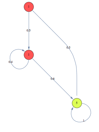
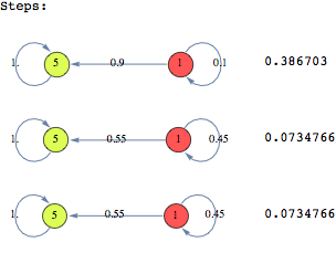
and let mcN be the Markov chain MC[{x,y},theta,ell] defined as follows
![]()

![]()
![]()
![]()
![]()

Example 2


![]()
![]()
![]()
![]()

![]()
![]()
![]()
![]()
![]()
Case Study: IPv4 Zero Conf Protocol
We consider the IPv4 Zero Conf protocol discussed in Example 10.5 [2]. For convenience, we report the same presentation of the protocol given in there.
The IPv4 zeroconf protocol is designed for a home local network of appliances (microwave oven, laptop, VCR, DVD player, etc.) each of which is supplied with a network interface to enable mutual communication. Such adhoc networks must be hot-pluggable and self- configuring. Among others, this means that when a new appliance (interface) is connected to the network, it must be configured with a unique IP address automatically. The zeroconf protocol solves this task in the following way. A host that needs to be configured randomly selects an IP address, U say, out of the 65,024 available addresses and broadcasts a message (called probe) saying “Who is using the address U?” If the probe is received by a host that is already using the address U, it replies by a message indicating that U is in use. After receiving this message the host to be configured will restart: it randomly selects a new address, broadcasts a probe, etc.
Due to message loss or a busy host, a probe or a reply message may not arrive at some (or all) other hosts. In order to increase the reliability of the protocol, a host is required to send n probes, each followed by a listening period of r time units. Therefore, the host can start using the selected IP address only after n probes have been sent and no reply has been received during n·r time units. Note that after running the protocol a host may still end up using an IP address already in use by another host, e.g., because all probes were lost. This situation, called address collision, is highly undesirable since it may force a host to kill active TCP/IP connections.
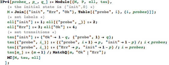
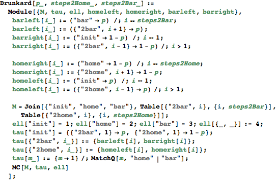
The following is a function that models the above potocol as a Markov chain, given the number of probes and the parameters ‘p’ and ‘q’ respectively for the probabilities of loosing the message or hitting an address that that is free to be used.
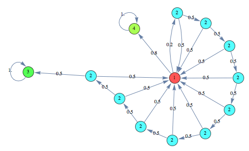
Here we have to instances of the above protocol with 10 and 2 succesive probes respectively.
![]()
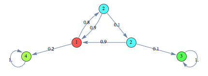
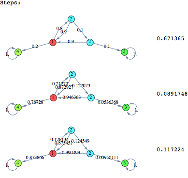
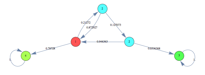
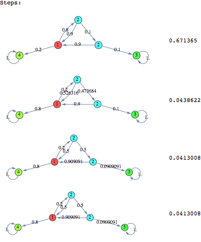
In the following we find a (sub-optimal) approximant of the protocol with 10 probes starting the search from an instance of the same protocol with only 2 probes
![]()
![]()
![]()
![]()
![]()
![]()
![]()
![]()
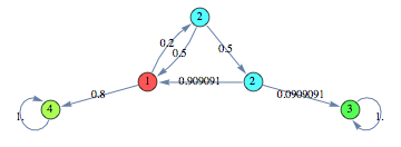
We can see that both the heuristics give very good results within few iterations. In this case the Averaged Marginal method seems to produce slightly better results, compared to the Averaged Expextation method.
Case Study: Drunkard’s Walk
A man walks along a four - block stretch of Park Avenue. If he is at corner 1, 2, or 3, then he walks to the left with probability p or to the right with probability (1-p). He continues until he reaches corner 4, which is a bar, or corner 0, which is his home. If he reaches either home or the bar, he stays there.
![]()
![]()

![]()
![]()
![]()
![]()

![]()
![]()
![]()
![]()
